Getting started

Simple search

This target combines a cosine term, a square term, and a constant.

The model searches with +, -, *, and /. To include the cosine used in the target, add unary_operators=["cos"].

import numpy as np

from pysr import PySRRegressor

X = 2 * np.random.randn(100, 5)
y = 2 * np.cos(X[:, 3]) + X[:, 0] ** 2 - 2
model = PySRRegressor(binary_operators=["+", "-", "*", "/"])
model.fit(X, y)
print(model)

Custom operator

A custom operator has a definition for the symbolic search and a callable for SymPy export and for evaluating equations. Here inv(x) = 1/x defines the Julia-side reciprocal operator, while extra_sympy_mappings gives that name its Python implementation.

import numpy as np

from pysr import PySRRegressor

X = 2 * np.random.randn(100, 5)
y = 1 / X[:, 0]
model = PySRRegressor(
    binary_operators=["+", "*"],
    unary_operators=["inv(x) = 1/x"],
    extra_sympy_mappings={"inv": lambda x: 1/x},
)
model.fit(X, y)
print(model)

The generic operators parameter replaces the separate unary_operators and binary_operators. Its integer keys specify arity, so a dictionary can describe unary, binary, and higher-arity operators. See the Operators of any arity section for this form.

Multiple outputs

A two-dimensional target makes the model multi-output. Here each column of y is the reciprocal of a different input feature, so the fitted model supplies one selected equation for each output.

import numpy as np

from pysr import PySRRegressor

X = 2 * np.random.randn(100, 5)
y = 1 / X[:, [0, 1, 2]]
model = PySRRegressor(
    binary_operators=["+", "*"],
    unary_operators=["inv(x) = 1/x"],
    extra_sympy_mappings={"inv": lambda x: 1/x},
)
model.fit(X, y)

Plotting an expression

After fitting the multi-output model, model.latex()[0] returns the LaTeX form of the selected equation for output 0.

model.latex()[0]

Use model.latex()[1] for output 1.

The plot below compares the target and prediction for output 0.

from matplotlib import pyplot as plt
plt.scatter(y[:, 0], model.predict(X)[:, 0])
plt.xlabel('Truth')
plt.ylabel('Prediction')
plt.show()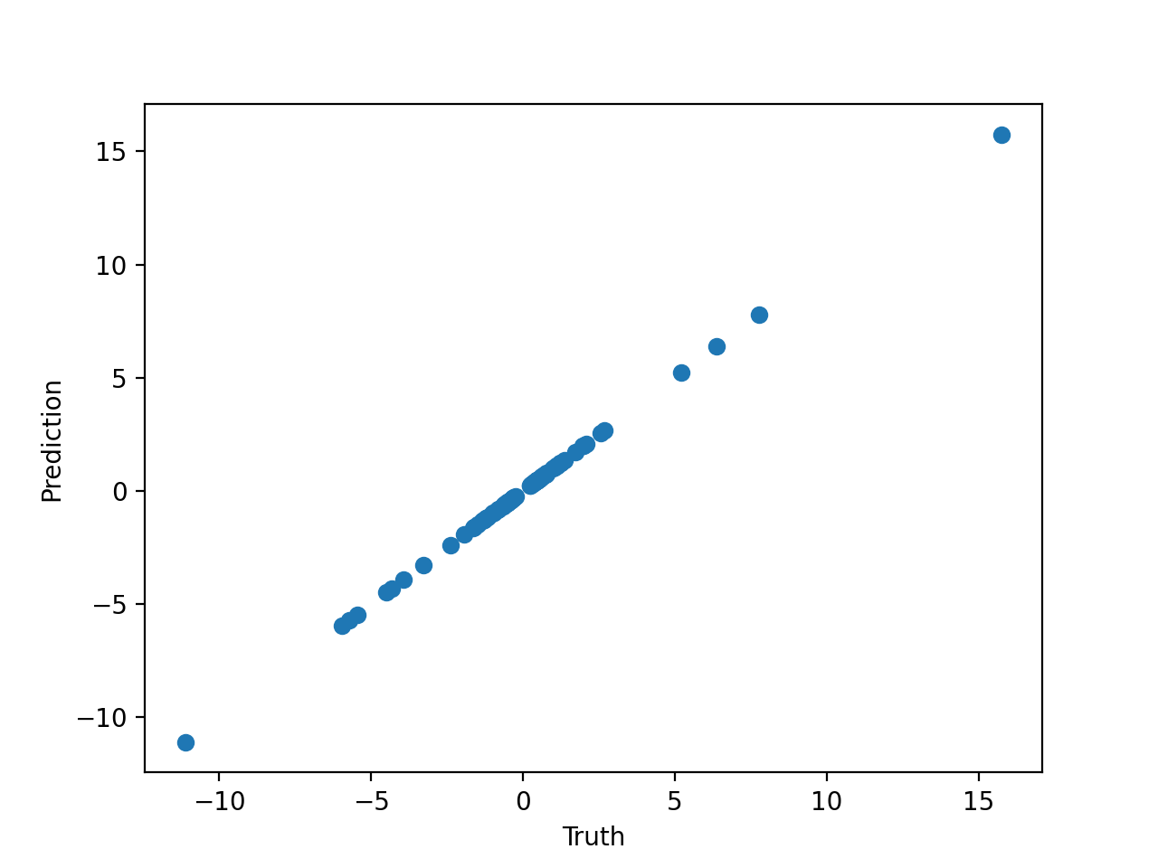

The index argument chooses a candidate equation from model.equations_. Pass it to predict, sympy, or latex to inspect or evaluate another candidate. For multiple outputs, provide one equation index per output in output order, then select the desired output column from the predictions.

Feature selection

Feature selection reduces the candidate input columns before symbolic regression. Set select_k_features=5 to use a random-forest preprocessor that retains up to five candidates. For structured high-dimensional data, the paper 2006.11287 discusses breaking the problem into smaller pieces before applying PySR.

The target in this example uses features 3 and 19.

import numpy as np

X = np.random.randn(300, 30)
y = X[:, 3]**2 - X[:, 19]**2 + 1.5

Configure feature selection in the model:

from pysr import PySRRegressor

model = PySRRegressor(
    binary_operators=["+", "-", "*", "/"],
    unary_operators=["exp"],
    select_k_features=5,
)

Fit the model to select the input columns before the search:

model.fit(X, y)

PySR prints the selected feature names before starting the search, for example:

Using features ['x3', 'x5', 'x7', 'x19', 'x21']

The names use zero-based column indices. This selection includes both target features, x3 and x19, plus three other candidates. The symbolic search uses only these retained columns.

Denoising

When per-observation weights are available, pass weights to fit and define elementwise_loss with the matching signature. Without weights, the function accepts (prediction, target). With weights, it accepts (prediction, target, weight). The weighted example uses elementwise_loss="myloss(x, y, w) = w * (x - y)^2". Pass a full custom objective as loss_function.

The denoise=True option preprocesses the targets with a Gaussian process before symbolic regression. Its predictions become the targets searched by PySR. Because this example passes no Xresampled, the predictions are made at the original rows in X.

The target combines an exponential term, two linear terms, and random noise:

import numpy as np

X = np.random.randn(100, 5)
noise = np.random.randn(100) * 0.1
y = np.exp(X[:, 0]) + X[:, 1] + X[:, 2] + noise

Create and fit the denoising model:

from pysr import PySRRegressor

model = PySRRegressor(
    binary_operators=["+", "-", "*", "/"],
    unary_operators=["exp"],
    denoise=True,
)
model.fit(X, y)
print(model)